Exhibit 6.5

Overview
Roys allow holders to benefit from the success of a Talent by granting them a monthly return corresponding to the economic performance of the Talent. To measure these performances, we emulate a Talent’s income via public and semi-public data that allows us to infer the Talents’ real income. For example, the number of sponsored posts on a Talent’s Instagram can be used to approximate that Talent’s income from brand deals.
From five to ten different types of data derived from Instagram, at the time of the Talent’s listing, the algorithm will generate a Gaussian of the talent’s revenue probabilities for the next 10 years.

Each month, the Talent’s position on the Gaussian is recalculated based on the Talent’s actual performance. The better the Talent’s economic performance is, the further to the right of the graph the Talent is. It is on this monthly recalculated basis that the yield is paid (today this return is framed between a minimum of 2% per year and a maximum of 50% per year of the nominal value of the Roy - $2.00).
If a user buys the same proportion of all the Talents on the platform, they will receive each year for 10 years on average a 7-8% return. (Average observed in 2023 - 8.27%) even though some may return much more or much less.
In order to demonstrate how the algorithm operates, the following is an example of the application of the algorithm social media influence of Talents.
We will first describe our methodology for quantitative talent valuation by breaking down revenue by social network, to understand the link between talent activity on social networks and their revenue. We will then describe our method of segmenting the different influencers and then describe our method of predicting future revenues. Finally we will see how to use the model to arrive at a robust valuation and other applications that derive from the structure of this model.
I. Description of the Influencer Valuation Model
a) The model
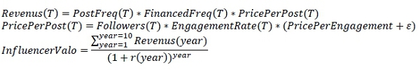
We model talent revenues on social networks as the direct sum of granular revenues. To illustrate this, let’s take a period T of 1 month, we can then break down the revenue over this period:
Revenus(T)=PostFreq(T)*FinancedFreq(T)*PricePerPost(T)
Where:
PostFreq = Number of posts on the social network over the period T,
FinancedFreq = Percentage of financed posts (i.e. content financed by a brand for the influencer to include in a post),
PricePerPost = Price for a funded publication
This last quantity is key for the modelling, it represents the amount that a brand is willing to pay for a publication by this influencer on the social network. It is explained as follows:
PricePerPost(T)=Followers(T)*EngagementRate(T)*(PricePerEngagement+ε)
Where:
Followers = Number of users on the social network following the influencer’s account,
EngagementRate = User engagement rate, also known as community. It is calculated as follows: number of likes plus the number of comments per publication divided by the number of Followers.
PricePerEngagement = Price brands are willing to pay per user following the influencer and being engaged.
We will see later how to estimate the PricePerEngagement parameter, and we will also justify this formulation in a quantitative way. It will depend for example on the country in which the influencer has the majority of his audience and on the quality of his audience. Finally, we integrate the random part of the PricePerPost in an Epsilon random variable for which we will see that the hypothesis of zero mean will be verified. It remains for us to determine the uncertainty thanks to the variance.
By using the influencer’s data on the social network and the actual market prices for the publications we can calibrate the revenue model. We will then describe the type of statistical modelling (Hierarchical Bayesian regression model) that we use to perform the calibration.
Once the revenue model is in place, we define a future period of 10 years over which we must predict the influencer’s revenue. To do this, we need to predict the value of the dynamic variables of the model, mainly the number of Followers and the engagement rate. We will see later on how we make this prediction based on a Bayesian auto-regression model.
Finally we have access to a valuation:

Where:
year = year over which we predict ({1,2,..,10})
r = rate at which future income is discounted
b) The Data available
For our modelling we opted for an unlimited subscription to Favikon (https://www.favikon.com/) a digital marketing decision support platform for Instagram that has a large amount of public data on the activity of influencers of all sizes by scrapping directly on the Instagram platform. We access this data via the API which allows us to extract large amounts programmatically.
We have used this platform to extract over 30,000 Instagram accounts located in Europe with at least 100,000 followers and not linked to a brand.
This gives us access to historical data on follower numbers and engagement rates. In addition, we have audience data such as follower location and demographic data. Finally, we also have textual data such as hashtags and mentions used in influencers’ publications.
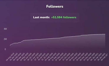
Below is an example of a major French influencer:
We also have access to a sample of pricing data (price per publication, price per story) from a French influencer agency coupled with pricing data from an online platform for digital marketing.
We will now describe our statistical approach to infer the parameters of the model using the data at our disposal.
II. Inference Methods
a) Segmentation
To separate the influencers into different groups, and thus analyse the importance of the separators in the model, we start by using the location of the audience by looking at the country with the largest proportion of the audience per influencer.
Then we use a separation based on the number of followers and the engagement rate as a quantitative variable. This separation is simply done in percentiles, so group ordered with equal proportion.

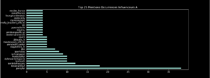
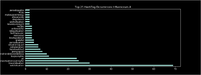
Finally, we define a sectoral segmentation using textual data composed of hashtags and mentions used by influencers in their publications. For each influencer, we create a table with the number of occurrences of each hashtag and mention. Below is an example of a table for influencer A:
We then normalise each influencer by dividing each table by the sum of the occurrences. The separation method we use is inspired by the Bag Of Words method see [4,5] used in Natural Language Processing consisting in creating a large matrix, where each row is the name of the influencer and the columns correspond to all the mentions (resp. hashtags) used at least once by at least one of the influencers. We therefore observe a very sparse matrix with a majority of zeros on each row except for the columns where for the influencer in question there is at least one occurrence.
These sparse matrices are also very large, so the dimension should be reduced. To do this, one method considered is principal component analysis see [3,4]. It would give groups directly, but it has the limitation of losing the interpretability of each component.
To overcome this problem we use an iterative method consisting of iteratively sorting the words by their total occurrences and then removing the words with the least occurrences and evaluating the total variance of the sample. When a final variance of at least 80% is reached, the process is stopped. This effectively reduces the size of the matrices (number of columns) while maintaining the information set.
We can then calculate measures of similarity between profiles by calculating the dot product between each profile. Finally we sort for a profile or a set of profiles selected as representative of a sector the most similar profiles. We can also create clusters that we will call sectors, by classical clustering methods such as K-Means, Hierarchical methods, etc.
b) Price per engagement
We will now describe the model we have developed to estimate the prices per engagement introduced in II.a. For this purpose, we have 25 prices per publication from a French talent management agency. These prizes are offered to brands to collaborate with the influencers that the agency manages. To this we add 30 awards per publication from an online platform known as the reference for brands, agencies and influencers directly.
We opted for a hierarchical Bayesian model, which has the advantages of delivering fully interpretable conclusions, allowing complete control over the different factors of variability, and expressing the uncertainty around each variable used as well as the predictions. In particular, it allows us to overcome the problem of overfitting with the help of the a priori that we impose, as well as to regularise the model that contains correlated variables. More information on the structure and details of these models can be found in [1,2,6,7].
We formulate from the equation introduced in II.a:
PricePerPost (T)=Followers (T)*EngagementRate (T)*(PricePerEngagement+ε)
The following hierarchical model:
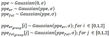
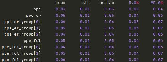
Where, ppe represents the price per commitment, we use a very conservative a priori centred in 0 with a low Sigma standard deviation. This allows us to regularise the model (strong evidence from the data will be needed to justify II.a). Next we want to see the effect of engagement rate and number of followers on ppe. We therefore create 3 groups for each as described in III.a.
The hierarchy is as follows ppe follows a normal distribution centred in 0, then ppe_er and ppe_fol follow normal distributions centred in ppe, finally for each group segmented in number of followers and engagement rate (i,j above) ppe_er_group[i] and ppe_fol_group[j] follow normal distributions centred in ppe_er and ppe_fol.
This leaves some variability from each group but still constrained to not deviate from the parent parameter ppe.
For each influencer coming from the agency prices we retrieve the quantitative values (number of influencers, engagement rate) as close as possible to the date of publication of the prices.
We also tried to add other variables such as sectors, growth, etc., however these variables do not add predictability or in a very uncertain way, moreover the number of points being limited we opted for a choice of stability and interpretability by keeping a parsimonious model.
Sigma is chosen as weak and then validated from a range by cross validation see [8]. We then separate the data into two parts, one part (In Sample) on which we regress the parameters and a second part (Out Of Sample) on which we evaluate the quality of the model.
Finally, we performed the MCMC inference, see [9], using Python as a programming language and the JAX library (https://jax.readthedocs.io/en/latest/) which allows to translate scientific models in a flexible way and very efficient in terms of computation time.
Below we find the parameters resulting from the inference. We observe very healthy a posteriori distributions centred around 0.05 with very moderate deviations from the mean. The MCMC chains are also very healthy as can be seen on the following graph (third quadrant).

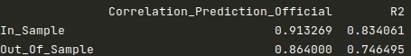
Below we find the correlations between predicted and actual values as well as the coefficient of determination. These values are very strong and stable on both In Sample and Out Of Sample.
Finally, below we find the links between final price predictions by publication and actual (official) values. We have added the confidence interval [1%,99%] of the model’s predictions (accessible through the Bayesian format) for each point. The model thus explains the vast majority of the variability with very reasonable accuracy.

We therefore inferred a strong link between the prices used by branders and the characteristics of influencers in France. The formulation is fully interpretable with a very moderate amount of variability. It will now be possible to use the characteristics of a new French influencer to determine a price per engagement (and the associated uncertainty) at any time on historical data for example, as well as future predictions of these characteristics.
We will now detail our future growth model which will allow us to give future predictions of these characteristics.
c) Regressive model for predicting future growth
As we introduced in II.a to predict future revenues we need to predict the dynamic variables of the revenue model. We start with the most important variable expressing the most variability over time, the number of followers.
To do this we define the following hierarchical Bayesian past-future growth regression model:
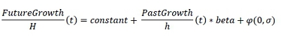
The hierarchy is as follows:

Where beta represents the relationship between past and future growth, H (resp. h) is the period over which future (resp. past) growth is calculated and constant represents the past-independent quantity in future growth. Again we use very conservative a priori centred in 0 with low Gamma and Alpha standard deviations. Finally, similar to II.b we want to see the effect of engagement rate and number of followers as well as the period h on beta. We therefore create 4 groups for each as described in III.a.
The hierarchy is as follows beta follows a normal distribution centred in 0, then beta_er, beta_fol and beta_h follow normal distributions centred in beta, and finally for each group segmented in number of followers, engagement rate and h (i,j,k above) beta_er_group [i], beta_fol_group [j] and beta_h_group follow normal distributions centred in beta_er, beta_fol and beta_h.
This leaves variability from each group but still constrained to not deviate from the parent parameter beta. The constant parameter follows an equivalent approach.
We used the 30,000 counts available to us over the period of about 2 years. This allowed us to calibrate the model on almost 220,000 points which we then normalise.
Finally, Gamma and Alpha are selected in the same way as Sigma in III.b.
Below we find the parameters resulting from the inference. We observe very healthy a posteriori distributions centred around 0.55 for beta and 0.01 for constant with very moderate deviations from the mean.
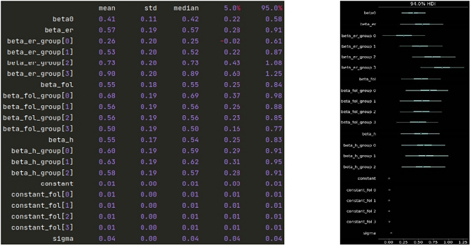
We can observe a strong impact of the engagement rate, the higher this rate is, the more past growth is linked to future growth. This confirms the intuition that the more the audience is engaged, the more the influencer is attractive, he creates value for his audience and thus attracts more people by trend effect. The number of followers also has a more moderate impact, the higher the number of followers, the less important the link between past and future growth. Indeed, intuitively, we can think that from a certain number of followers the account becomes less personalized and reaches a certain threshold. Finally, the period over which we calculate the growth has a lesser effect, which we will keep in mind when we predict over several time steps and will therefore help us to stabilise our predictions even more.
As for the constant parameter, we find the fact that social networks are in a period of strong growth as we introduced in I. There is therefore a macro trend independent of the characteristics of the influencers.
Below we find the correlations between predicted and actual values as well as the coefficient of determination. These values are very strong and stable on the two samples In Sample and Out Of Sample.

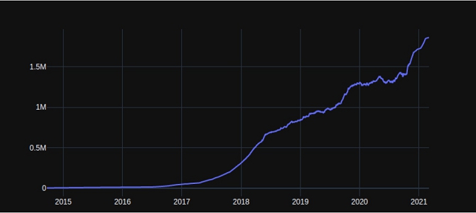
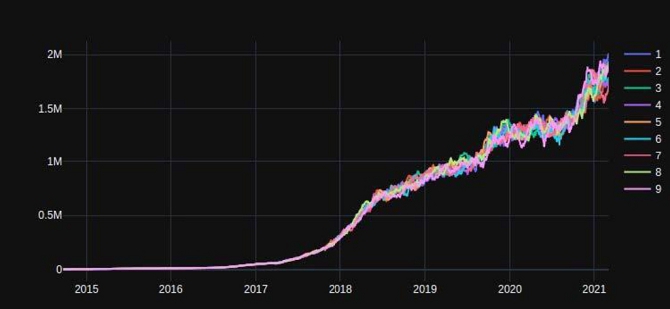
Finally below we look at the final follower predictions on 4 influencers. By observing the actual values up to a certain time, then using the predictive model we apply to several consecutive future steps. We obtain robust future predictions with a good control of uncertainty. (blue: actual values, yellow: predicted values, [purple-red]: confidence interval on predictions)
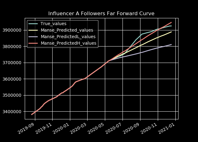
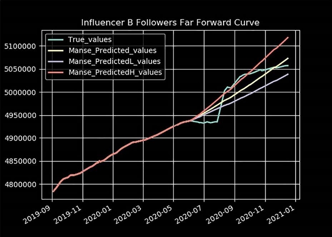


It is therefore now possible to predict a future trajectory of the number of followers with a controlled level of uncertainty.
In order to obtain a valuation of an influencer we can now join each part of the model and thus define this valuation in expectation (average) and also estimate the moments and confidence intervals around this expectation. This is detailed in the next section.
d) Valuation by future discounted income
Recall the formulation introduced in II:
We have described how to infer the price per engagement and the future evolution of the number of followers. We now need to formulate the post frequency, the frequency of funded posts and the engagement rate.
From the observations obtained in our database of influencers we can obtain the post frequency as the average over the last months of the number of posts, we add around this average the measured standard deviation of this estimator. We proceed in the same way for the financial post frequency, for each observed post we analyse the textual content if a brand is mentioned or if it is an official partnership then we consider this post as a funded post.
Thus we obtain a mean value and a standard deviation of this measure. We can therefore rephrase these two quantities as follows:
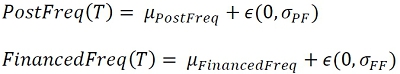
Although we observe a negative relationship of the engagement rate as a function of the number of followers in an absolute way when comparing thousands of influencers’ accounts, by focusing on the temporal dynamics of this variable for each influencer independently we do not find a strong enough relationship to be justified in the model.
Indeed, starting from an engagement rate value, the temporal evolution of the number of followers for an influencer does not express a strong enough link of temporal predictability with the evolution of the engagement rate. Therefore, we use a modelling similar to PostFreq and FinancedFreq:

Finally, let us recall the formulation obtained previously for the number of followers:
MonthNdays representing the number of days for month T (value for H).
We thus arrive at the valuation expressed as follows:

For the sake of clarity we have renamed PricePerEngagement to include Epsilon.
This quantity is by definition a random variable for which the expectation is easily accessible and is the average expected price.

To obtain the degree of uncertainty, it will be appropriate, for example, to simulate the trajectories by Monte Carlo or to use a semi-explicit formulation coupled with a dynamic programming method and thus obtain a distribution around the average price.
Finally, the choice of the rate at which future revenues are discounted depends on the use and can also integrate the uncertainty around the average price as a measure of risk, which will be translated into a minimum rate of return on investment for example.
III. Applications and Integration in Manse
As our valuation method is entirely systematic, it opens up a wide range of applications. Indeed, by accessing tens of thousands of influencer profiles, we can for example observe and study the past evolution of the value of a talent. To do this we apply the valuation formula to each historical point and thus obtain the valuation history.
Below we find, for an influencer A, his past trajectory of average values:
We can also observe the influence of the uncertainty around the different variables of the model. Below we observe for example for this same influencer a sample of historical values by simulating the uncertainty around the Price Per Commitment.
One example is the nowcasting method, which consists of assessing the value of an unobservable quantity in a continuous manner, at each point in time by simply observing the social network variables at time t and applying the revenue formula. We then obtain a real time estimate of an influencer’s income, even though it is not directly observable in an official way.
Thanks in particular to the historical trajectory, it is possible to estimate returns on investment as well as the associated risks. By applying classical methods one can also assess the correlation with other asset classes such as equities or government bonds etc., by aligning the historical price series of equities and government bonds with those of the influencer.
By comparing the different influencers within their sectors, for example, we can assess the performance of an influencer relative to its sector by studying all the historical curves in comparison. It is also possible to detect high potential talents, or to detect trends among sectors.
This method will also be used when introducing talent to the Manse platform in the following way:
1 - Select an Influencer A.
2 - Obtain at least 2 years of official revenue from the influencer.
3 - Apply the revenue model to the period of official revenue obtained in 2 and
refine the parameters of the model accordingly.
4 - Apply the Valuation model with the new refined parameters.
5 - Follow the evolution of the valuation in Nowcasting once the talent is on the platform.
Conclusion
It should be remembered that to date, there is no method of valuation by expected future income of an individual, and even less so for the category of influencers on social networks. This type of innovative talent in a very recent and fast-growing sector of activity constitutes an important and complex challenge in terms of valuation.
We have introduced an innovative method based on quantitative modelling of key performance factors used by brand owners to model influencer revenues. In particular, we developed a strong understanding of the relationship between talent activity on social networks and their revenues through robust modelling based on a large number of data sets. Following this, by modelling the dynamics of the talent’s activity and audience, we built a rigorous predictive model of future revenues supported by a validation on a large number of real points.
Finally, thanks to the systematic and quantitative nature of the valuation model and the data driven segmentation, we have introduced a number of applications that we are implementing within Manse allowing us to propose innovative products and offering the user an understanding and a controlled level of risk thanks to the complete measurement of uncertainty.
Références
[1] Greg M. Allenby, Peter E. Rossi, Robert E. McCulloch(2005) Hierarchical Bayes Models: A Practitioners Guide.
[2] Roger Levy (2012) - Probabilistic Models in the Study of Language, Chapter8, Hierarchical Models.
[3] Cosma Shalizi, Carnegie Mellon University, lecturel2, Chapter18, Principal Components Analysis.
[4] B F Ljungberg, (2017), Dimensionality reduction for bag-of-words models: PCA vs LSA.
[5] Steven Bird, Ewan Klein, and Edward Loper. Natural Language Processing with Python. O’Reilly Media, 2009.
[6] Rossi, Peter E., Greg M. Allenby and Robert E. McCulloch (2005), Bayesian Statistics and Marketing, New York: Wiley.
[7] Andrews, Rick , Asim Ansari, and Imran Currim (2002) “Hierarchical Bayes versus finite mixture conjoint analysis models: A comparison of fit, prediction, and partworth recovery,” journal of Marketing Research, 87-98
[8] Sebastian Raschka,(2018), Model Evaluation, Model Selection, and Algorithm Selection in Machine Learning
[9] Matthew D. Hoffman, Andrew Gelman, (2011), The No-U-Turn Sampler: Adaptively Setting Path Lengths in Hamiltonian Monte Carlo
[10] Brown D, Hayes N (2008) Influencer Marketing: Who Really Influences Your Customers? (Elsevier/ButterworthHeinemann), ISBN 9780750686006, URL https://books.google.frIbooks?id=250V.515MIC.
[11] Nora Lisa Ewers, (2017) #sponsored - Influencer Marketing on Instagram An Analysis of the Effects of Sponsorship Disclosure, Product Placement, Type of Influencer and their Interplay on Consumer Responses
[12] Glucksman M (2017) The rise of social media influencer marketing on lifestyle branding: A case study of lucie fink. Elon Journal of Undergraduate Research in Communications 8(2):77-87
[13] Zietek N (2016) Influencer marketing: the characteristics and components of fashion influencer marketing.
[14] Berthon, P. R., Pitt, L. F., Plangger, K., & Shapiro, D. (2012). Marketing meets Web 2.0, social media, and creative consumers: Implications for international marketing strategy. Business horizons, 55(3), 261-271.
[15] Brown, D., & Hayes, N. (2008). Influencer Marketing: Who really influences your customers?. Routledge.
[16] Djafarova, E., & Rushworth, C. (2017). Exploring the credibility of online celebrities’ Instagram profiles in influencing the purchase decisions of young female users. Computers in Human Behavior, 68, 1-7.
[17] Gageler, L., & Van der Schee, J. (2016). Product Placement on Social Media: a study on how Generation Y’s brand perception and purchase intention are influenced.
[18] Facebook developper framework, https://developers.facebook.com/
Annexes
A. Digital Marketing: Official Figures
A. 1. Monthly active users on Instagram
Source: Demandsage

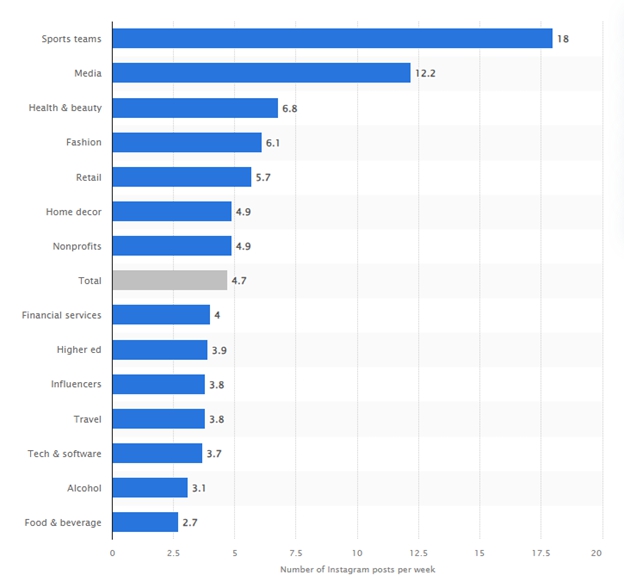
A. 2. Number of Instagram sponsored posts per category in 2023, in millions
Source: Statistica
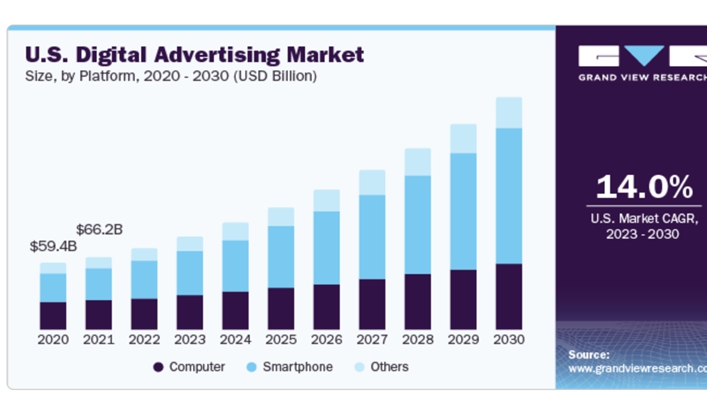
A. 3. Digital marketing market sizes in billions of USD
Source: Grandviewresearch
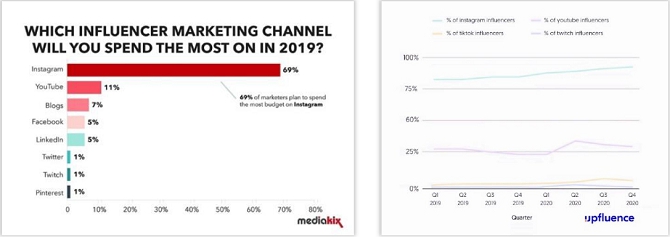
B. Digital Marketing: Official surveys


C. Digital Marketing: Sample Posts